Run the full PREP

In this example we show how to run the full PREP pipeline on a noisy EEG recording using PrepPipeline, inspect which channels it flags as bad, and visualize the effect of cleaning.

# Authors: The PyPREP developers
# SPDX-License-Identifier: MIT

First we import what we need for this example.

import matplotlib.pyplot as plt
import mne
import numpy as np
from mne.datasets import eegbci

from pyprep.prep_pipeline import PrepPipeline

Load some data

We use subject 4, run 1 from the PhysioNet BCI2000 (eegbci) dataset. This is a fairly noisy recording, which makes it a good candidate for demonstrating PREP. The data are 64-channel EEG sampled at 160 Hz.

mne.set_log_level("WARNING")

edf_fpath = eegbci.load_data(subjects=4, runs=1, update_path=True)[0]
raw = mne.io.read_raw_edf(edf_fpath, preload=True)

# The eegbci data ships with non-standard channel names, so we fix them and
# attach a standard montage (PREP needs sensor positions to interpolate).
eegbci.standardize(raw)
montage = mne.channels.make_standard_montage("standard_1005")
raw.set_montage(montage)

# Keep an untouched copy of the original data for a before/after comparison.
raw_before = raw.copy()

Set PREP parameters and run the pipeline

• ref_chs / reref_chs: the channels used to build, and to be cleaned by, the robust average reference. "eeg" means “all EEG channels”.

• line_freqs: the line-noise frequencies to remove. This is a US recording, so line noise sits at 60 Hz and its harmonics below Nyquist.

RANSAC is stochastic, so the set of detected bad channels depends on the random seed. We fix the seed to make this example reproducible. Note the seed is not a small, hand-picked number like 42: such “magic” seeds are easy to (even unconsciously) cherry-pick for a flattering result. Instead we drew a single high-entropy value once via secrets.randbits(31) and hardcoded it (31 bits keeps it within the range accepted by NumPy’s legacy RandomState, which is what random_state ultimately feeds). See NumPy’s RNG guidance: https://numpy.org/doc/stable/reference/random/index.html

random_state = 466171092

sfreq = raw.info["sfreq"]
prep_params = {
    "ref_chs": "eeg",
    "reref_chs": "eeg",
    "line_freqs": np.arange(60, sfreq / 2, 60),
}

prep = PrepPipeline(raw, prep_params, montage, random_state=random_state)
prep.fit()

<pyprep.prep_pipeline.PrepPipeline object at 0x7a1ee7f834d0>

Inspect the detected bad channels

PREP records the channels it considers bad at several points in the pipeline. The most useful summaries are:

• noisy_channels_original: bad channels found on the raw data, before any robust referencing.

• interpolated_channels: channels that were bad after robust referencing and were therefore replaced by a spherical-spline interpolation from their neighbors.

• still_noisy_channels: channels that remain bad even after interpolation. After interpolating, PREP runs noisy-channel detection one final time on the cleaned data; anything flagged here could not be rescued (e.g. interpolation left it looking atypical relative to its neighbors, or it only became an outlier once the data were re-referenced). These channels are reported, not re-interpolated, so you can decide whether to drop them or handle them manually. An empty list is the ideal outcome.

We coerce the names to plain str purely for tidy printing: some detection methods return channel names as numpy.str_ (e.g. RANSAC, which indexes a NumPy array of names), so the raw lists can mix 'Fp1' and np.str_('F7').

original_bads = sorted(map(str, prep.noisy_channels_original["bad_all"]))
interpolated = sorted(map(str, prep.interpolated_channels))
still_noisy = sorted(map(str, prep.still_noisy_channels))

print(f"Bad channels (original): {original_bads}")
print(f"Interpolated channels:   {interpolated}")
print(f"Still noisy afterwards:  {still_noisy}")

Bad channels (original): ['AF3', 'AF4', 'AF7', 'AF8', 'F6', 'F7', 'F8', 'FT8', 'Fp1', 'Fp2', 'Fpz']
Interpolated channels:   ['AF3', 'AF4', 'AF7', 'AF8', 'AFz', 'C5', 'CP3', 'CP4', 'F3', 'F5', 'F6', 'F7', 'F8', 'FC1', 'FC3', 'FC5', 'FT7', 'FT8', 'Fp1', 'Fp2', 'Fpz', 'P2', 'P4', 'P7', 'Pz', 'T10', 'T8', 'TP7']
Still noisy afterwards:  ['C4', 'C6', 'Fp1', 'Fpz']

Visualize the effect of PREP

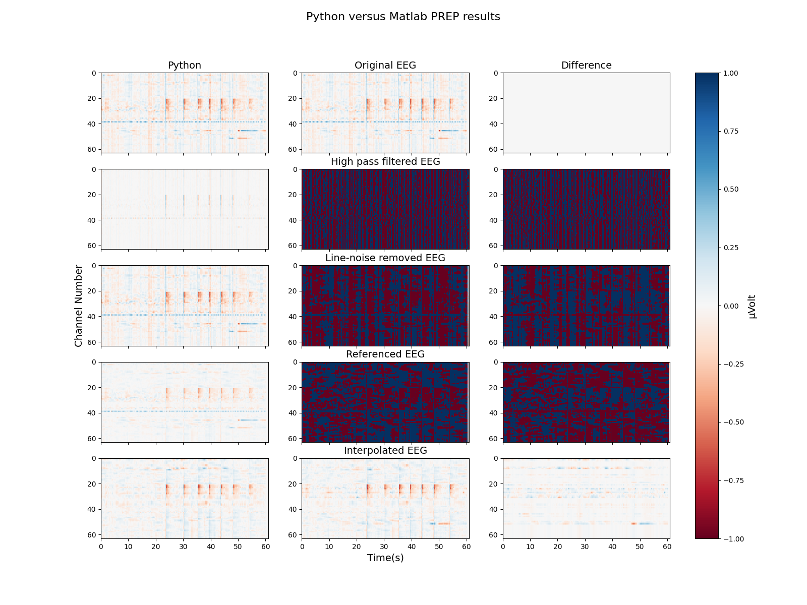
A power spectral density (PSD) plot is a compact way to see what PREP did. Compared to the raw data, the cleaned data should show the 60 Hz line-noise peak removed and a tighter spread across channels (bad channels no longer stick out, having been interpolated from their neighbors).

fig, axs = plt.subplots(
    1, 2, figsize=(12, 4), sharex=True, sharey=True, constrained_layout=True
)

raw_before.compute_psd(fmax=80).plot(axes=axs[0], show=False)
axs[0].set_title("Before PREP")

prep.raw.compute_psd(fmax=80).plot(axes=axs[1], show=False)
axs[1].set_title("After PREP")

Text(0.5, 1.0, 'After PREP')

A time-domain view before/after

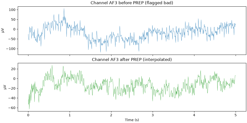
The PSD summarizes the whole recording but hides what happens to individual channels. The clearest thing to see in the time domain is interpolation: a channel that PREP flagged as bad is replaced by an estimate from its neighbors. (Line-noise removal and re-referencing also change the traces, but their effect is subtler and better appreciated in the PSD above.)

Below we plot the first interpolated channel over a short window. The “before” trace is the untouched recording (so it still contains drift and line noise), while the “after” trace is the fully cleaned, interpolated signal.

ch = interpolated[0]
tmax = 5.0  # seconds
window = raw_before.times <= tmax
times = raw_before.times[window]

before = raw_before.get_data(picks=ch)[0, window] * 1e6  # volts -> microvolts
after = prep.raw.get_data(picks=ch)[0, window] * 1e6

fig, axs = plt.subplots(2, 1, figsize=(10, 5), sharex=True, constrained_layout=True)
axs[0].plot(times, before, lw=0.5)
axs[0].set(title=f"Channel {ch} before PREP (flagged bad)", ylabel="μV")
axs[1].plot(times, after, lw=0.5, color="tab:green")
axs[1].set(
    title=f"Channel {ch} after PREP (interpolated)",
    ylabel="μV",
    xlabel="Time (s)",
)

[Text(0.5, 1.0, 'Channel AF3 after PREP (interpolated)'), Text(27.055888888888894, 0.5, 'μV'), Text(0.5, 18.503588541666666, 'Time (s)')]

The cleaned recording in prep.raw is a standard mne.io.Raw object, so you can carry on with the rest of your analysis pipeline (epoching, filtering, ICA, etc.) directly from there.